Theoretical Analysis of Metapopulation Models of Landscape Dynamics. Hal Caswell and I developed spatially explicit ecological models to explore how the relative spatial and temporal scales of biotic interactions (competition, predation), dispersal and disturbance interact to control coexistence, the structure of communities and the dynamics of landscapes. We used cellular automata (CA) models as descriptions of ecological interactions in space and time. CA models are essentially discretized versions of reaction-diffusion models and are closely related to patch-occupancy models for metapopulation dynamics. Each cell in the model provides a patch that can support populations of 1 or more species and are color coded accordingly. Our work has focused primarily on 2 species models of competition and predation (see Figures). In the models we can alter the rate of competitive exclusion (or other biotic interactions), dispersal rates (scale and colonization probability), and the size and frequency of disturbance. We have used the models to explore a number of specific problems, including the importance of dispersal in patchy environments, the effects of habitat fragmentation on biodiversity, the relationship between biotic and substrate heterogeneity in landscape dynamics, and the contrast of CA models with the corresponding nonspatial patch-occupancy model. Our analyses include several non-spatial or mean-field properties (state and species frequencies, mean alpha and beta diversities, interspecific associations, and turnover rates) as well as a suite of explicitly spatial methods (fractal dimensions and other scaling relationships, 2-dimensional spectral analysis, etc.). This work has been supported by the National Science Foundation and the Office of Naval Research
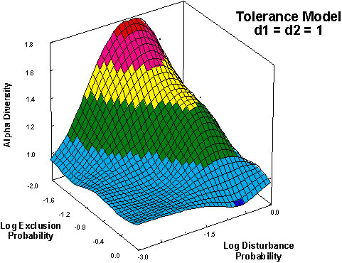
Fig. 3. The average diversity within patches as a function of the rate of competitive exclusion and the frequency of disturbance for a tolerance model of competition. Alpha diversity is calculated after the frequencies of sp1 and sp2 reach an equilibrium. In this example, the dispersal abilities of both species are equal (d1=d2).
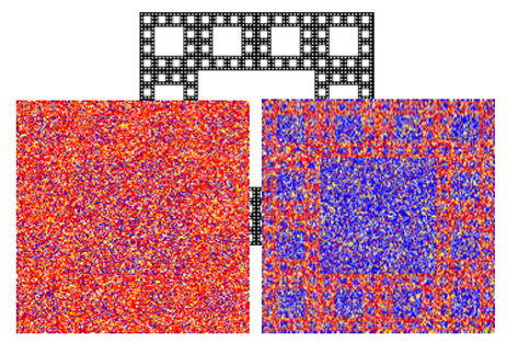
Fig. 4. The effect of a heterogeneous landscape on patch dynamics and spatial distributions of species. In the previous examples, the landscape was homogeneous with all patches identical - the parameters were the same for each patch. In this example the landscape is heterogeneous such that patches differ with respect to the parameters. The heterogeneity is shown by the black and white fractal in the background - competition occurs more rapidly in the white patches than in the black. Competitive exclusion rates are 10%(left panel) or 100%(right panel) faster in the white patches compared to the black. All other parameters are the same. When the difference in competitive exclusion rates are small, it is difficult to detect the heterogeneity from the distribution of species (patch colors). As the difference in dynamics between patches increases, the physical heterogeneity is more apparent in the distribution of species.


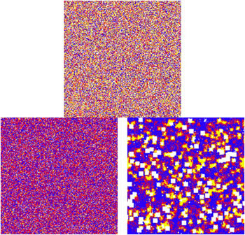
Fig. 1. Three landscape of 65,536 (256x256) homogeneous patches where multiple species can coexist. Color codes indicate which species are present in each patch (white = open patch, blue = species 1 the dominant competitor, yellow = species 2 the subordinate competitor but better disperser, red = both species present - eventually species 1 will outcompete species 2 in each patch). The top panel represents the starting conditions (random distribution of patches with 0, 1 or 2 species). The 2 lower panels show the distribution of patch types after 2000 iterations. Both lower panels have the same parameters (competitive exclusion rates, dispersal rates and disturbance frequency). The only difference is that disturbance size varies. On the left all disturbances are the size of a single patch, on the right disturbance occurs on 3 scales (1x1, 3x3 and 10x10 patches). A time series of the landscape changes is shown below.
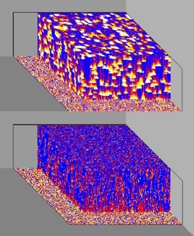
Fig. 2. A time series of landscapes stacked on top of one another. This shows how the landscape changes over 200 iterations of the CA model. The bottom landscape represents the random initial conditions. All subsequent landscapes were cut away to better visualize the patch dynamics (time moving up). Note that in the upper panel with variable size disturbance, the largest disturbances are initially colonized from the edges by the inferior competitor (yellow) followed by the superior competitor (red for both species in patch) and eventually sp1 outcompetes sp2 leaving only sp1 in the patch (blue). Similar sequences play out for the smaller disturbances but are more difficult to see.
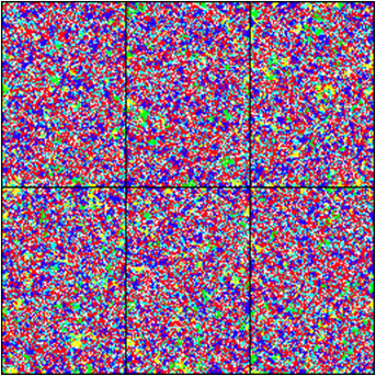
Fig. 5. An individual based CA. This model differs from the others in that each patch (cell) can support only 1 individual. The landscape depicts the distribution of 6 species (colors) across 6 independent subtidal rock walls. The parameters for the transition matrix were derived from 20 years of photo-monitoring of natural rock wall communities in the Gulf of Maine by Ken Sebens. We are exploring the relative importance of local dispersal (within a wall) and inter-wall dispersal in effecting the dynamics and spatial distributions of species within these subtidal assemblages